9.1 Australian Marriage Survey

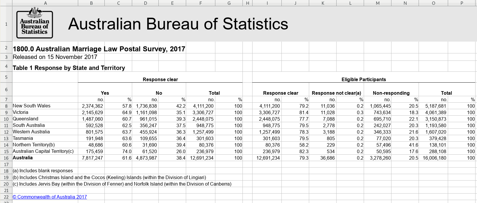
These are the results of a survey in 2017 by the Australian Bureau of Statistics that asked, “Should the law be changed to allow same-sex couples to marry?”
There are two tables with structures that are similar but different. Download the file. Original source.
9.1.1 The full code listing
cells <- xlsx_cells(smungs::ozmarriage)
formats <- xlsx_formats(smungs::ozmarriage)

table_1  <-
  cells %>%
  dplyr::filter(sheet == "Table 1", row >= 5L, !is_blank) %>%
  mutate(character = str_trim(character)) %>%
  behead("up-left", "population") %>%
  behead("up-left", "response") %>%
  behead("up", "unit") %>%
  behead("left", "state") %>%
  arrange(row, col) %>%
  select(row, data_type, numeric, state, population, response, unit) %>%
  spatter(unit) %>%
  select(-row)

state <-
  cells %>%
  dplyr::filter(sheet == "Table 2",
                row >= 5L,
                col == 1L,
                !is_blank,
                formats$local$font$bold[local_format_id]) %>%
  select(row, col, state = character)

table_2 <-
  cells %>%
  dplyr::filter(sheet == "Table 2",
                row >= 5L,
                !is_blank) %>%
  mutate(character = str_trim(character)) %>%
  behead("up-left", "population") %>%
  behead("up-left", "response") %>%
  behead("up", "unit") %>%
  behead("left", "territory") %>%
  enhead(state, "up-left") %>%
  arrange(row, col) %>%
  select(row, data_type, numeric, state, territory, population, response,
         unit) %>%
  spatter(unit) %>%
  select(-row)

all_tables <- bind_rows("Table 1" = table_1, "Table 2" = table_2, .id = "sheet")
all_tables
## # A tibble: 1,176 x 7
## sheet state population response `%` no. territory
## <chr> <chr> <chr> <chr> <dbl> <dbl> <chr>
## 1 Table 1 New South Wales Eligible Participants Non-responding 20.5 1065445 <NA>
## 2 Table 1 New South Wales Eligible Participants Response clear 79.2 4111200 <NA>
## 3 Table 1 New South Wales Eligible Participants Response not clear(a) 0.2 11036 <NA>
## 4 Table 1 New South Wales Eligible Participants Total 100 5187681 <NA>
## 5 Table 1 New South Wales Response clear No 42.2 1736838 <NA>
## 6 Table 1 New South Wales Response clear Total 100 4111200 <NA>
## 7 Table 1 New South Wales Response clear Yes 57.8 2374362 <NA>
## 8 Table 1 Victoria Eligible Participants Non-responding 18.3 743634 <NA>
## 9 Table 1 Victoria Eligible Participants Response clear 81.4 3306727 <NA>
## 10 Table 1 Victoria Eligible Participants Response not clear(a) 0.3 11028 <NA>
## # … with 1,166 more rows9.1.2 Step by step
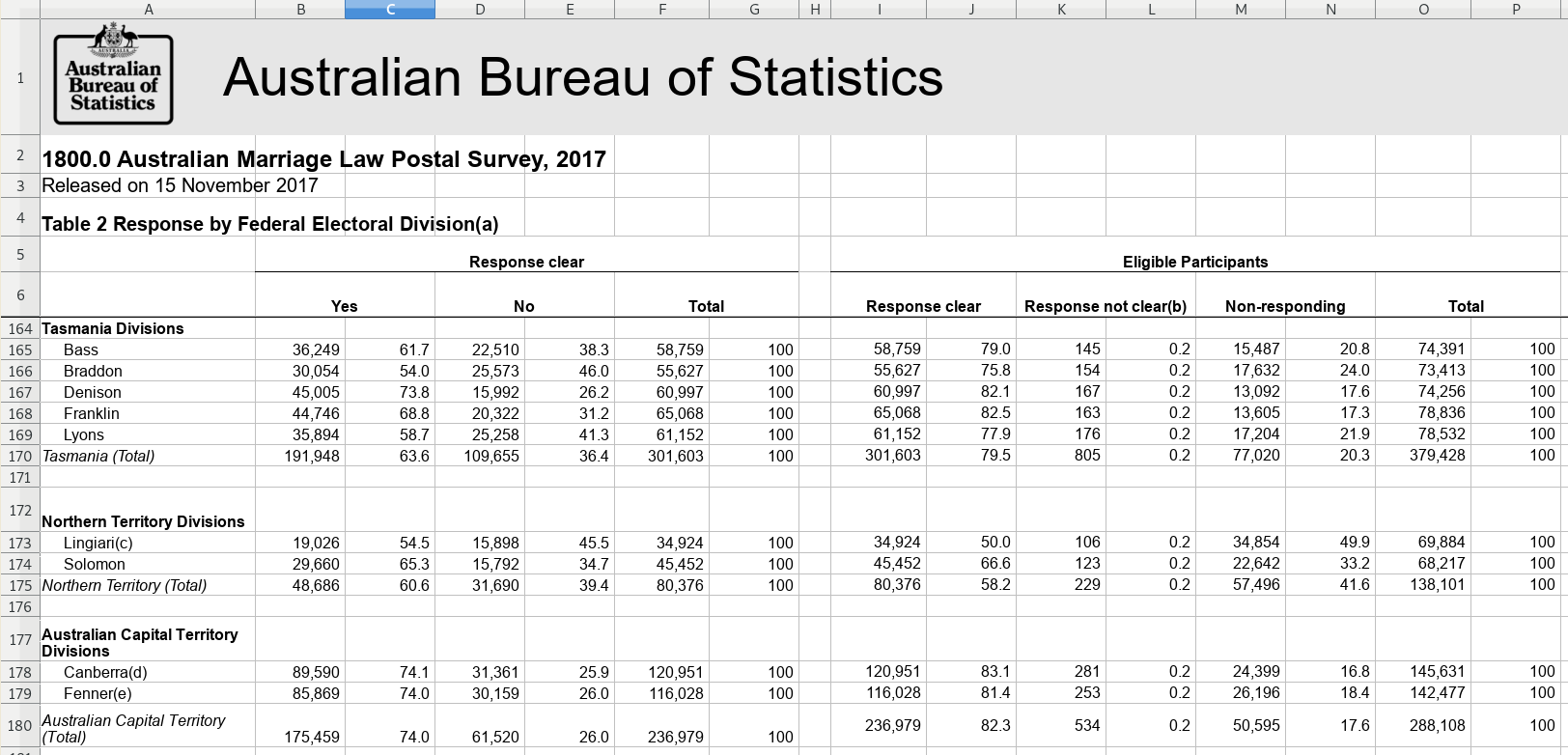
9.1.2.1 Table 1
The first rows, up to the column-headers, must be filtered out. The trailing rows below the table will be treated us row-headers, but because there is no data to join them to, they will be dropped automatically. That is handy, because otherwise we would have to know where the bottom of the table is, which is likely to change with later editions of the same data.
Apart from filtering the first rows, the rest of this example is ‘textbook’.
cells <- xlsx_cells(smungs::ozmarriage)

table_1  <-
  cells %>%
  dplyr::filter(sheet == "Table 1", row >= 5L, !is_blank) %>%
  mutate(character = str_trim(character)) %>%
  behead("up-left", "population") %>%
  behead("up-left", "response") %>%
  behead("up", "unit") %>%
  behead("left", "state") %>%
  arrange(row, col) %>%
  select(row, data_type, numeric, state, population, response, unit) %>%
  spatter(unit) %>%
  select(-row)

table_1
## # A tibble: 63 x 5
## state population response `%` no.
## <chr> <chr> <chr> <dbl> <dbl>
## 1 New South Wales Eligible Participants Non-responding 20.5 1065445
## 2 New South Wales Eligible Participants Response clear 79.2 4111200
## 3 New South Wales Eligible Participants Response not clear(a) 0.2 11036
## 4 New South Wales Eligible Participants Total 100 5187681
## 5 New South Wales Response clear No 42.2 1736838
## 6 New South Wales Response clear Total 100 4111200
## 7 New South Wales Response clear Yes 57.8 2374362
## 8 Victoria Eligible Participants Non-responding 18.3 743634
## 9 Victoria Eligible Participants Response clear 81.4 3306727
## 10 Victoria Eligible Participants Response not clear(a) 0.3 11028
## # … with 53 more rows9.1.2.2 Table 2
This is like Table 1, broken down by division rather than by state. The snag is
that the states are named in the same column as their divisions. Because the
state names are formatted in bold, we can isolate them from the division names.
With them out of the way, unpivot the rest of the table as normal, and then use
enhead() at the end to join the state names back on.
Since tables 1 and 2 are so similar structurally, they might as well be joined into one.
cells <- xlsx_cells(smungs::ozmarriage)
formats <- xlsx_formats(smungs::ozmarriage)

state <-
  cells %>%
  dplyr::filter(sheet == "Table 2",
                row >= 5L,
                col == 1L,
                !is_blank,
                formats$local$font$bold[local_format_id]) %>%
  select(row, col, state = character)

table_2 <-
  cells %>%
  dplyr::filter(sheet == "Table 2",
                row >= 5L,
                !is_blank) %>%
  mutate(character = str_trim(character)) %>%
  behead("up-left", "population") %>%
  behead("up-left", "response") %>%
  behead("up", "unit") %>%
  behead("left", "territory") %>%
  enhead(state, "up-left") %>%
  arrange(row, col) %>%
  select(row, data_type, numeric, state, territory, population, response,
         unit) %>%
  spatter(unit) %>%
  select(-row)

all_tables <-
  bind_rows("Table 1" = table_1, "Table 2" = table_2, .id = "sheet") %>%
  select(sheet, state, territory, population, response, `%`, no.)
all_tables
## # A tibble: 1,176 x 7
## sheet state territory population response `%` no.
## <chr> <chr> <chr> <chr> <chr> <dbl> <dbl>
## 1 Table 1 New South Wales <NA> Eligible Participants Non-responding 20.5 1065445
## 2 Table 1 New South Wales <NA> Eligible Participants Response clear 79.2 4111200
## 3 Table 1 New South Wales <NA> Eligible Participants Response not clear(a) 0.2 11036
## 4 Table 1 New South Wales <NA> Eligible Participants Total 100 5187681
## 5 Table 1 New South Wales <NA> Response clear No 42.2 1736838
## 6 Table 1 New South Wales <NA> Response clear Total 100 4111200
## 7 Table 1 New South Wales <NA> Response clear Yes 57.8 2374362
## 8 Table 1 Victoria <NA> Eligible Participants Non-responding 18.3 743634
## 9 Table 1 Victoria <NA> Eligible Participants Response clear 81.4 3306727
## 10 Table 1 Victoria <NA> Eligible Participants Response not clear(a) 0.3 11028
## # … with 1,166 more rows