3 Pivot tables
This part introduces pivot tables. Tidyxl and unpivotr come into their own here, and are (as far as I know) the only packages to acknowledge the intuitive grammar of pivot tables.
Pivot tables are ones with more than one row of column headers, or more than one column of row headers, or both (and there can be more complex arrangements). Tables in that form take up less space on a page or a screen than ‘tidy’ tables, and are easier for humans to read. But most software can’t interpret or traverse data in that form; it must first be reshaped into a long, ‘tidy’ form, with a single row of column headers.
It takes a lot of code to reshape a pivot table into a ‘tidy’ one, and the code has to be bespoke for each table. There’s no general solution, because it is ambiguous whether a given cell is part of a header or part of the data.
There are some ambiguities in ‘tidy’ tables, too, which is why most functions for reading csv files allow you to specify whether the first row of the data is a header, and how many rows to skip before the data begins. Functions often guess, but they can never be certain.
Pivot tables, being more complex, are so much more ambiguous that it isn’t reasonable to import them with a single function. A better way is to break the problem down into steps:
- Identify which cells are headers, and which are data.
- State how the data cells relate to the header cells.
The first step is a matter of traversing the cells, which is much easier if
you load them with the tidyxl package, or
pass the table through as_cells() in the
unpivotr package. This gives you a table
of cells and their properties; one row of the table describes one cell of the
source table or spreadsheet. The first two properties are the row and column
position of the cell, which makes it easy to filter for cells in a particular
region of the spreadsheet. If the first row of cells is a header row, then you
can filter for row == 1.
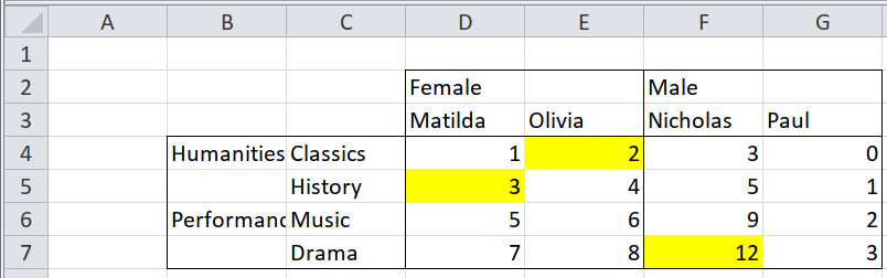
Here is an example of a pivot table where the first two rows, and the first two columns, are headers. The other cells contain the data. First, see how the cells are laid out in the source file by importing it with readxl.
path <- system.file("extdata", "worked-examples.xlsx", package = "unpivotr")
original <- read_excel(path, sheet = "pivot-annotations", col_names = FALSE)
## New names:
## * `` -> ...1
## * `` -> ...2
## * `` -> ...3
## * `` -> ...4
## * `` -> ...5
## * ...## # A tibble: 6 x 6
## ...1 ...2 ...3 ...4 ...5 ...6
## <chr> <chr> <chr> <chr> <chr> <chr>
## 1 <NA> <NA> Female <NA> Male <NA>
## 2 <NA> <NA> Matilda Olivia Nicholas Paul
## 3 Humanities Classics 1 2 3 0
## 4 <NA> History 3 4 5 1
## 5 Performance Music 5 6 9 2
## 6 <NA> Drama 7 8 12 3Compare that with the long set of cells, one per row, that tidyxl gives. (Only a few properties of each cell are shown, to make it easier to read).
cells <- xlsx_cells(path, sheets = "pivot-annotations")
select(cells, row, col, data_type, character, numeric) %>%
print(cells, n = 20)## # A tibble: 32 x 5
## row col data_type character numeric
## <int> <int> <chr> <chr> <dbl>
## 1 2 4 character Female NA
## 2 2 5 blank <NA> NA
## 3 2 6 character Male NA
## 4 2 7 blank <NA> NA
## 5 3 4 character Matilda NA
## 6 3 5 character Olivia NA
## 7 3 6 character Nicholas NA
## 8 3 7 character Paul NA
## 9 4 2 character Humanities NA
## 10 4 3 character Classics NA
## 11 4 4 numeric <NA> 1
## 12 4 5 numeric <NA> 2
## 13 4 6 numeric <NA> 3
## 14 4 7 numeric <NA> 0
## 15 5 2 blank <NA> NA
## 16 5 3 character History NA
## 17 5 4 numeric <NA> 3
## 18 5 5 numeric <NA> 4
## 19 5 6 numeric <NA> 5
## 20 5 7 numeric <NA> 1
## # … with 12 more rowsA similar result is obtained via unpivotr::as_cells().
## New names:
## * `` -> ...1
## * `` -> ...2
## * `` -> ...3
## * `` -> ...4
## * `` -> ...5
## * ...## # A tibble: 36 x 4
## row col data_type chr
## <int> <int> <chr> <chr>
## 1 1 1 chr <NA>
## 2 1 2 chr <NA>
## 3 1 3 chr Female
## 4 1 4 chr <NA>
## 5 1 5 chr Male
## 6 1 6 chr <NA>
## 7 2 1 chr <NA>
## 8 2 2 chr <NA>
## 9 2 3 chr Matilda
## 10 2 4 chr Olivia
## 11 2 5 chr Nicholas
## 12 2 6 chr Paul
## 13 3 1 chr Humanities
## 14 3 2 chr Classics
## 15 3 3 chr 1
## 16 3 4 chr 2
## 17 3 5 chr 3
## 18 3 6 chr 0
## 19 4 1 chr <NA>
## 20 4 2 chr History
## # … with 16 more rows(One difference is that read_excel() has filled in some missing cells with
blanks, which as_cells() retains. Another is that read_excel() has
coerced all data types to character, whereas xlsx_cells() preserved the
original data types.)
The tidyxl version is easier to traverse, because it describes the position of each cell as well as the value. To filter for the first row of headers:
## # A tibble: 2 x 4
##     row   col character numeric
##   <int> <int> <chr>       <dbl>
## 1     2     4 Female         NA
## 2     2     6 Male           NA
Or to filter for cells containing data (in this case, we know that only data cells are numeric)
## # A tibble: 16 x 3
##      row   col numeric
##    <int> <int>   <dbl>
##  1     4     4       1
##  2     4     5       2
##  3     4     6       3
##  4     4     7       0
##  5     5     4       3
##  6     5     5       4
##  7     5     6       5
##  8     5     7       1
##  9     6     4       5
## 10     6     5       6
## 11     6     6       9
## 12     6     7       2
## 13     7     4       7
## 14     7     5       8
## 15     7     6      12
## 16     7     7       3
By identifying the header cells separately from the data cells, and knowing exactly where they are on the sheet, we can associated the data cells with the relevant headers.
To a human it is intuitive that the cells below and to the right of the header
Male represent males, and that ones to the right of and below the header
Postgraduate qualification represent people with postgraduate qualifications,
but it isn’t so obvious to the computer. How would the computer know that the
header Male doesn’t also relate to the column of cells below and to the left,
beginning with 2?
This section shows how you can express the relationships between headers and data cells, using the unpivotr package.